Burrows-Wheeler, Coronavirus, & Bayes

A Bioinformatics Pipeline to Detect & Understand COVID Mutants

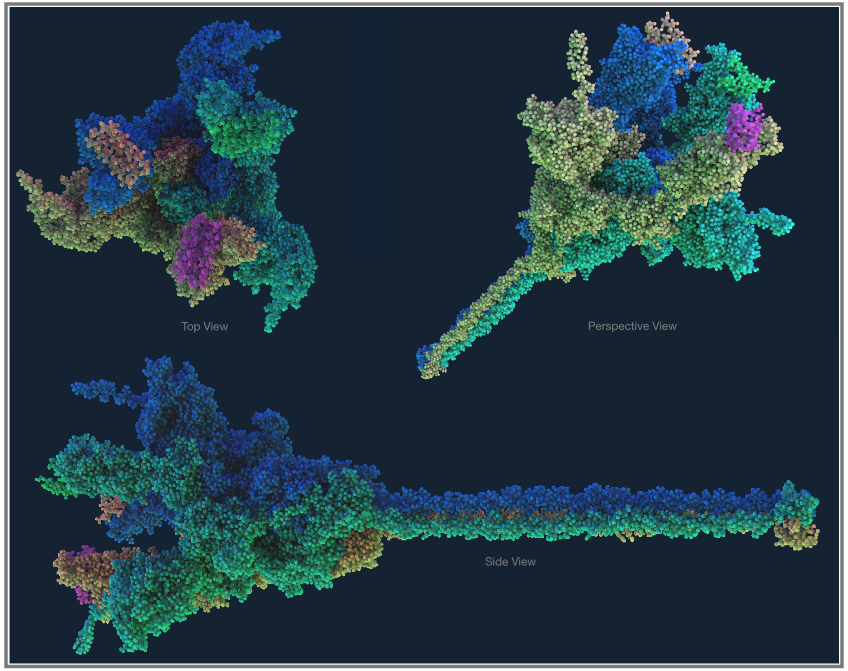
Fig 1. Molecular Structure with UK Mutant SARS-CoV-2 Docked to Human Receptor

As the pandemic runs its course, tracking genetic mutations has gained mainstream coverage. Officially, in the line of work we call bioinformatics, finding and understanding mutations is known as Variant Calling. In the same way every person is different from others (except twins), an individual virus can have variations in their genome; when a lot of these genetic variations accumulate between the virus we detected originally and what we find months later in a faraway town, we can say that we have a new strain of the virus. The Coronavirus which we’re now calling SARS-CoV-2 was first detected in Wuhan中国, so the genetic sequencing data from here is used as the base reference genome, and we measure mutations for the virus detected everywhere else against this; a coronavirus genome from a few towns away might only have a couple letters of the genome different from the Wuhan data, while something that’s travelled to the other side of the world after being transmitted through many people, climates, and even treatments, might now have acquired many more genetic variants compared to the original data.

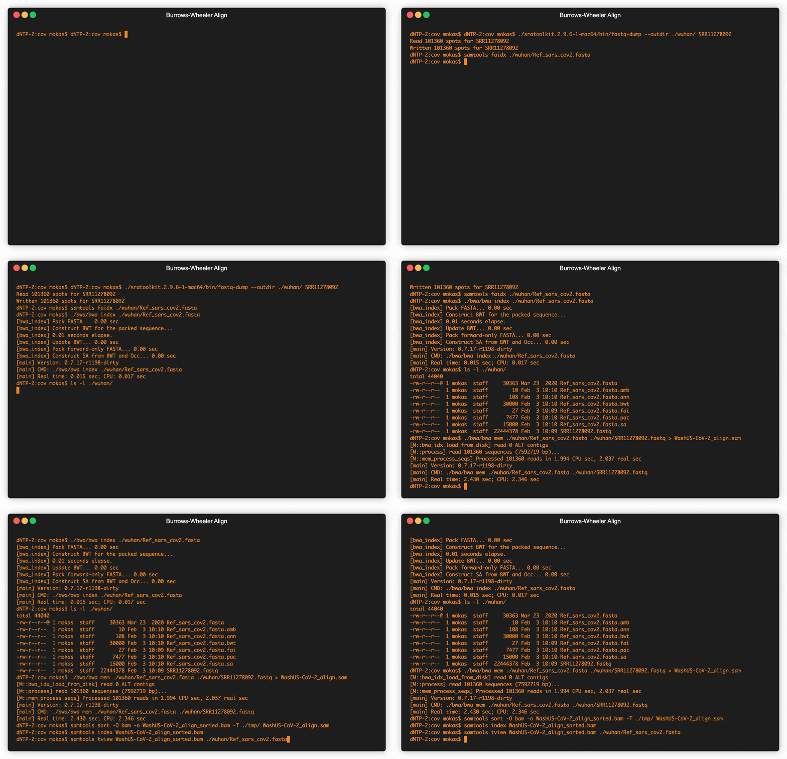
Fig 2. Retrieving raw COVID data from SRA & creating alignment maps

Data from viruses sequenced all across the world are uploaded into one of several databases (Table 1), this data is generated directly from machines by Illumina, Oxford Nanopore, or Life Technologies. When turning the molecules in genetic code into digital files these machines create strings that can be a few hundred letters in length to several thousand, but never the entire genome of the virus in a single string. A standardized file format called fastq holds all the strings from a single sample, including some quality data from the machine doing the sequencing. These strings are in no particular order, and first need to be mapped together to get the complete genome. Pretty much the standard way to create these genetic maps uses a technique invented in Palo Alto back in the early 90s by  Michael Burrows and David Wheeler. The Burrows–Wheeler Transform was mostly just used in data compression, until around 2010 when computational biologists began to use it to align genomes together.

Table 1.

SRA: Sequence Read Archive -Open Access

ENA: European Nucleotide Archive -Open Access

GISAID: Global Initiative on Sharing All Influenza Data -Private

Heng Li, now a professor at Harvard (amongst other things) has created the most commonly used alignment algorithm (amongst other things) with BWA. This algorithm is super easy to use, and will get us results that are more than good enough.

git clone https://github.com/lh3/bwa.git
cd bwa
make

BWA takes fastq files containing samples, along with a fasta file containing a reference genome to map the strings contained in our fastq file. Reference genomes are usually put out by the scientific wing of a National Government, Regional Organizations, and some Universities. We’ll get our Wuhan Coronavirus Reference genome from the National Center for Biotechnology Information hosted by the US Federal government. A good sample to run against the Wuhan reference is the Washington state outbreak that happened early in the US, the fastq data for this is also hosted by the NCBI at their Sequence Read Archive. In the animated terminal above (Fig 2.) we see the commands needed to create our mapped genome from our input files, including retrieving the data from the databases . If you’d like to skip all that, we’re hosting both the reference genome, and the completed alignment map over at Lucid Align. We’ll be using the bam file to detect our mutations, and we can also browse the genome of this Washington state outbreak sample using any sequence alignment viewer.

Fig 3. Detecting Mutations with Neural Networks

But before going on to variant calling this first sample let’s just prepare another sample while we’re making these alignment maps. Let’s do a more recent outbreak, from Kent, UK; which is far from Wuhan & the Washington sample, in both time & space. Retrieving the samples from the European Nucleotide Archive can be done from this link or from the shell.

git clone https://github.com/enasequence/enaBrowserTools.git
cd python3
enaDataGet.py -f fastq -m -d [output_directory] ERR4659819

Creating the mapped genome from the Kent, UK outbreak is done the exact same way as with the Washington state outbreak, and now both files can be browsed directly with an alignment viewer. More importantly now we can run the variant detection and see all the mutations in each of these samples compared to the original Wuhan reference genome. Variant callers are an area of hot development for folks working on bioinformatics algorithms & tools. Traditionally, Bayesian methods have been most reliable, but are hard-coded for specific organisms or need the settings dialed-in to get the correct sensitivity to specificity. This is so that we don’t get too many false-positives, while at the same time don’t miss any real mutations. In the last couple of years deep convolutional neural networks have really made a splash in variant calling, where now images are created almost similar to those we see from alignment viewers, and those images are used to train, and then have the neural network make the call on whether there is a mutation in a given section of the alignment map as we make our way down the entire map.

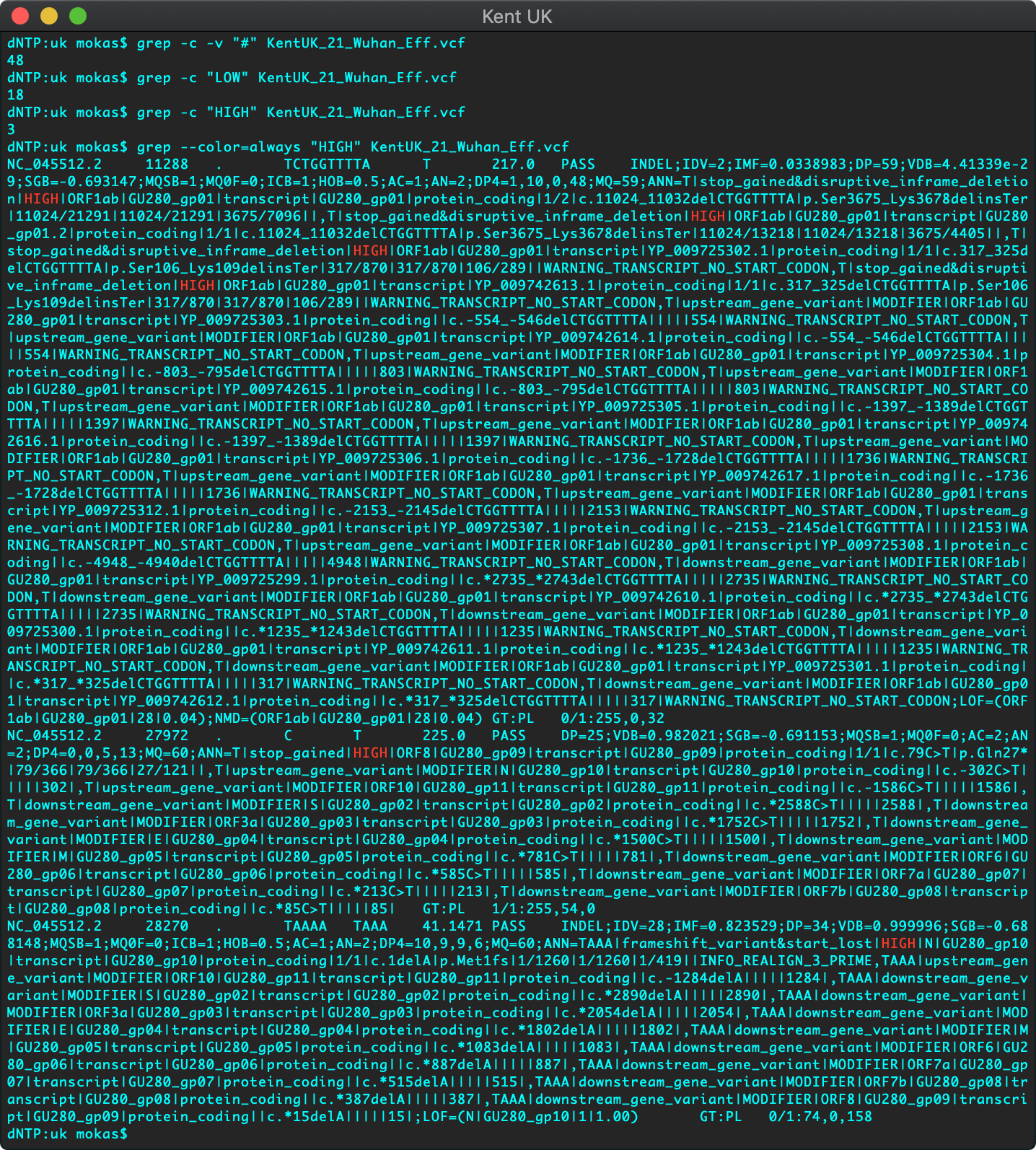
Fig 4. Annotated Mutations of Kent UK Strain B.1.1.7

Bayesian variant callers are fairly simple to install, whereas the DCNN callers will need, in our case, Nvidia cuda drivers, and of course a machine with those GPUs. You could use Magnolia Fig 3., the super-cool neural network based caller that Leo van Driel helped write B-), but for this post we are going to use the built-in caller that comes with samtools written by the previously mentioned Heng Li.

bcftools mpileup -Ou -f <ref.fasta> <sample1.bam> | bcftools call -vmO z -o <study.vcf.gz>

After running any variant caller, we’re left with a vcf file, which is just a list of positions in a genome where the sample has a mutation compared to the reference, it might be good to just look at the file format specifications to understand how these vcf files will be used moving forward. We can use the allotted fields in the vcf format to annotate, that is give meaning & context to each of the mutations we detect in the genome. For this sample we’ve used SnpEff which makes life super easy by boiling all of the predicted effects of each of the mutations we detected into 3 simple categories, high impact, low, and moderate.

We can see in Fig 4. that running a standard Bayesian variant caller we detected a total of 48 mutations in the Kent UK sample. However, there might be some false-positives in there, it’s always better to be a bit more sensitive than to miss things. Let’s focus on the high impact mutations, things that will change the 3D structure of coronavirus. Looks like we only have 3 of those, all highlighted in red (Fig 4.), at genomic positions, 11288, 27972, and 28270. The VCF file we generated also contains data on which amino acids within the protein structure were changed to what, we can use that information to make the changes in our molecular structure, which in this case we’ve done with a current tool under development.

Fig 5. Molecular Structure Editor

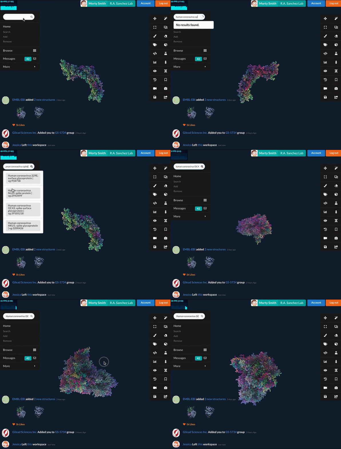
Mutations which change the molecular structure are super important because that is more likely to make things behave differently, this can mean it attaches to human receptors more tightly, interacts with antibodies and drugs differently, because remember at the core of how molecules behave is the old mantra “form equals function.”