Mapping the Quaternary Landscape

Building a Machine Learning System for Protein Complex Prediction

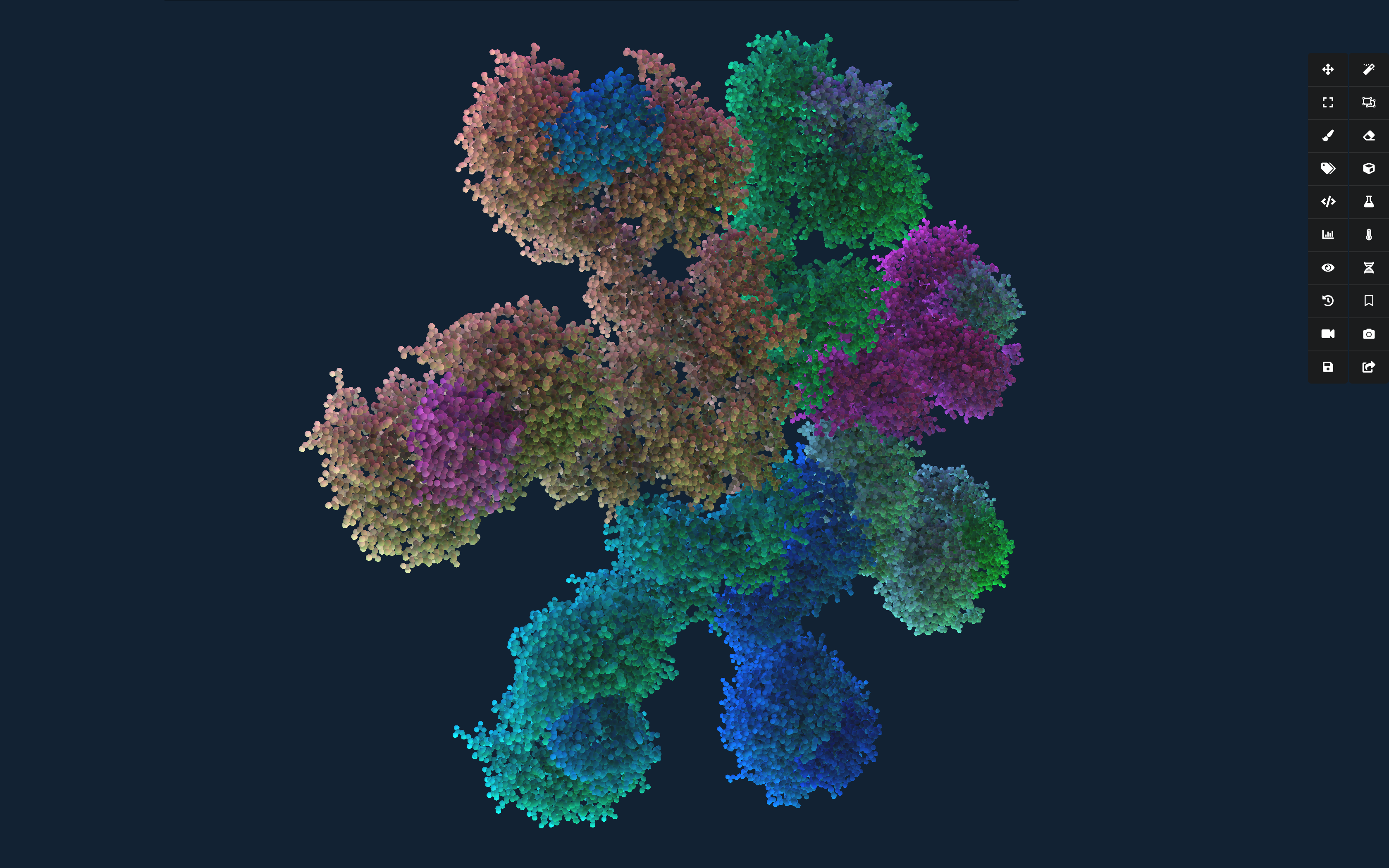
Proteins rarely work alone. Life happens when they come together — little machines that fit and unfit, join and dissolve, like a village of parts in constant conversation. Predicting the shape of one protein has been a milestone, AlphaFold gave us a breathtaking atlas of monomer structures; predicting how they assemble into complexes feels like the next step. Most fold into shapes that only make sense once you see how they fit together with others.

That’s the project the team at Jäntra has been working on: building a machine learning system for quaternary structure prediction. Instead of looking at one structure in isolation, the idea is to model how multiple structures interact, forming assemblies that actually do the work of life.

There’s no single data stream that tells the whole story. Structures from the PDB, predictions from AlphaFold, interaction maps from cryo-EM, evolutionary signals from sequences — each one is like a partial view through frosted glass. Machine learning, especially deep neural networks, gives us a way to blend these perspectives, to reason across modalities. The hard part is the scale and fluidity. Complexes can be huge, dynamic, and conditional.

Our starting approach and can be summerized by the following bottom-up strategy for quaternary structure prediction:

1. Start with a closed world:

Pick an organism like E. coli, where we already have tons of experimental + predicted structures in the AlphaFold DB.

We can simply use the AlphaFold Protein Structure Database API to grab our desired subset of predicted individual structures.

2. Bucketize monomers:

Cluster proteins into functional or structural groups (could be sequence families, Pfam domains, structural folds, GO annotations, etc.). This helps tame the combinatorial explosion — you’re not checking every protein against every other.

We can start with some basics using LibTorch

#include <torch/torch.h>

// --- Amino Acids + tensorizer ---
static const std::string AA = "ACDEFGHIKLMNPQRSTVWY";
static std::unordered_map<char,int> aa2idx = []{
  std::unordered_map<char,int> m;
  for (int i=0;i<(int)AA.size();++i) m[AA[i]]=i;
  return m;
}();
torch::Tensor seq_to_tensor(const std::string& seq, int max_len=512){
  auto t = torch::zeros({1, max_len}, torch::kLong);
  int L = std::min<int>(seq.size(), max_len);
  for (int i=0;i<L;++i) t[0][i] = aa2idx.count(seq[i]) ? aa2idx[seq[i]] : 20;
  return t;
}

// ---  Simple CNN embedder ---
struct SeqCNN : torch::nn::Module {
  torch::nn::Embedding emb{nullptr};
  torch::nn::Conv1d c1{nullptr}, c2{nullptr};
  torch::nn::Linear fc{nullptr};
  SeqCNN(int vocab=21, int ed=32, int out=256){
    emb = register_module("emb", torch::nn::Embedding(vocab, ed));
    c1  = register_module("c1", torch::nn::Conv1d(torch::nn::Conv1dOptions(ed,64,5).padding(2)));
    c2  = register_module("c2", torch::nn::Conv1d(torch::nn::Conv1dOptions(64,128,5).padding(2)));
    fc  = register_module("fc", torch::nn::Linear(128, out));
  }
  torch::Tensor forward(torch::Tensor x){
    auto e = emb->forward(x).transpose(1,2);       // [B,ed,L]
    auto h = torch::relu(c1->forward(e));
    h = torch::relu(c2->forward(h));               // [B,128,L]
    h = torch::adaptive_max_pool1d(h,1).squeeze(-1); // [B,128]
    return torch::nn::functional::normalize(fc->forward(h),
             torch::nn::functional::NormalizeFuncOptions().p(2).dim(1));
  }
};

We can now create a compact CNN embedding for each individual protein sequence, and then use K-means clustering to determine the buckets they are placed into.

// Read sequences
  std::vector<std::string> ids, seqs;
  for (auto& entry : fs::directory_iterator(fasta_dir)){
    if (!entry.is_regular_file()) continue;
    if (entry.path().extension() != ".fa" && entry.path().extension() != ".fasta") continue;
    auto id = entry.path().stem().string();
    auto seq = load_fasta_seq(entry.path());
    if (!seq.empty()){ ids.push_back(id); seqs.push_back(seq); }
  }
  if (ids.empty()){ std::cerr << "No FASTA found.\n"; return 1; }

  // Embed sequences
  SeqCNN encoder(21, 32, 256);
  encoder->eval(); // untrained: fine for clustering; replace with trained weights later
  std::vector<torch::Tensor> rows; rows.reserve(seqs.size());
  for (auto& s : seqs) rows.push_back(encoder->forward(seq_to_tensor(s,512)));
  auto X = torch::cat(rows, 0); // [N,256]

  // K-means clustering
  torch::manual_seed(42);
  int64_t N = X.size(0), D = X.size(1);
  auto centroids = X.index_select(0, torch::randperm(N).slice(0,0,K)).clone(); // [K,D]
  for (int it=0; it<20; ++it){
    auto dist = (X.pow(2).sum(1,true)) + (centroids.pow(2).sum(1).unsqueeze(0)) - 2*X.matmul(centroids.t());
    auto assign = std::get<1>(dist.min(1)); // [N]
    auto newC = torch::zeros_like(centroids);
    auto counts = torch::zeros({K}, torch::kFloat32);
    for (int i=0;i<N;++i){ int k = assign[i].item<int>(); newC[k] += X[i]; counts[k] += 1; }
    for (int k=0;k<K;++k) if (counts[k].item<float>()>0) newC[k] /= counts[k];
    centroids.copy_(newC);
  }
  auto finalDist = (X.pow(2).sum(1,true)) + (centroids.pow(2).sum(1).unsqueeze(0)) - 2*X.matmul(centroids.t());
  auto finalAssign = std::get<1>(finalDist.min(1));

  // Write mapping id -> bucket
  std::ofstream out(out_tsv);
  out << "id\tbucket\n";
  for (int i=0;i<N;++i) out << ids[i] << "\t" << finalAssign[i].item<int>() << "\n";
  std::cerr << "Wrote " << out_tsv << " with " << N << " rows.\n";
  return 0;

Why use K-Means?
The simple answer is, because it’s well understood and a good place to start the journey. If we have a set of protein structures from a model organism, \(((x_1, x_2, \dots, x_n))\), where each \((x_i \in \mathbb{R}^d)\) is a vector representation of a protein chain or domain. Then we can group these into \((k)\) functional or structural “buckets,” \((\mathcal{S} = \{ S_1, S_2, \dots, S_k \})\), so that proteins in the same bucket are structurally similar.

The objective is to minimize the within-cluster sum of squares (WCSS):

Here, \((\mu_i)\) is the centroid (average embedding) of cluster \((S_i)\):

where \((|S_i|)\) is the number of proteins in cluster \((S_i)\).
Intuitively, each cluster represents a structural “theme” and can also be viewed as minimizing the average pairwise distance between proteins inside each cluster:

with the equivalence given by:

K-means becomes a way of organizing the raw geometry of protein space, turning thousands of structures into a handful of interpretable groups we can later test for possible interactions. But much of this may result in quatranery structures we already know about, so we need to begin testing between our buckets.

3. Test for intra-bucket complexes:

Proteins in the same bucket are more likely to form homomers or closely related assemblies. You can start small here, validating known complexes (ribosomal proteins, polymerases, etc.).

4. Expand to inter-bucket pairs:

Once you have confidence, test cross-bucket interactions. This is where you might discover novel or less obvious complexes.

5. Layer in ML:

The buckets become priors or constraints for your machine learning model: instead of feeding the model the entire proteome, you give it “likely interaction neighborhoods.”

This approach we believe is similar to reducing a huge search space into manageable islands, then letting the model explore the coastlines where those islands might connect.

It’s a very different framing from AlphaFold-Multimer (which is trained end-to-end on complexes), but it’s a neat exploratory approach that could complement it: let the data itself suggest which assemblies to test.

You’re always walking a line between overfitting on the static snapshots we have, and missing the living reality where things are constantly in flux. Still, the effort feels worthwhile. These assemblies are the choreography of biology, and computational models can help us glimpse their dance. It’s equal parts engineering and humility — trying to learn patterns without pretending we can pin them down once and for all.